Housing Data Pipeline

Overview

For my NUS data engineering module, I worked in a five-person team to build an end-to-end pipeline for analysing Singapore’s housing market.

Our team used Airflow to orchestrate extraction, transformation, loading, model training, and report generation. The main modelling goal was to predict house prices from property characteristics and economic indicators. PostgreSQL acted as the data warehouse for the staged and analysis-ready data. My work focused on Python data cleaning and transformation, model experimentation, the Airflow environment, and the PropertyGuru scraper.

Pipeline

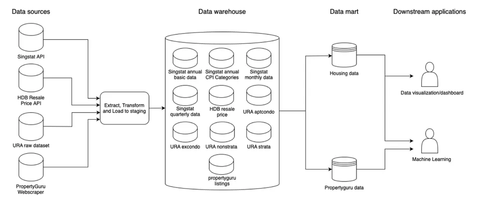
The pipeline combines four sources:

• HDB resale data: The data.gov.sg API provides more than 900,000 public-housing transactions.
• URA transactions: Spreadsheets provide recent private-property transactions because the available interface does not support reliable bulk extraction.
• SingStat indicators: Public APIs provide exchange rates, interest rates, CPI, unemployment, income, and inflation at monthly, quarterly, and annual frequencies.
• PropertyGuru listings: The Selenium scraper collects current asking prices and property attributes.

The sources have different update cycles and constraints, so we use separate ingestion tasks for each.

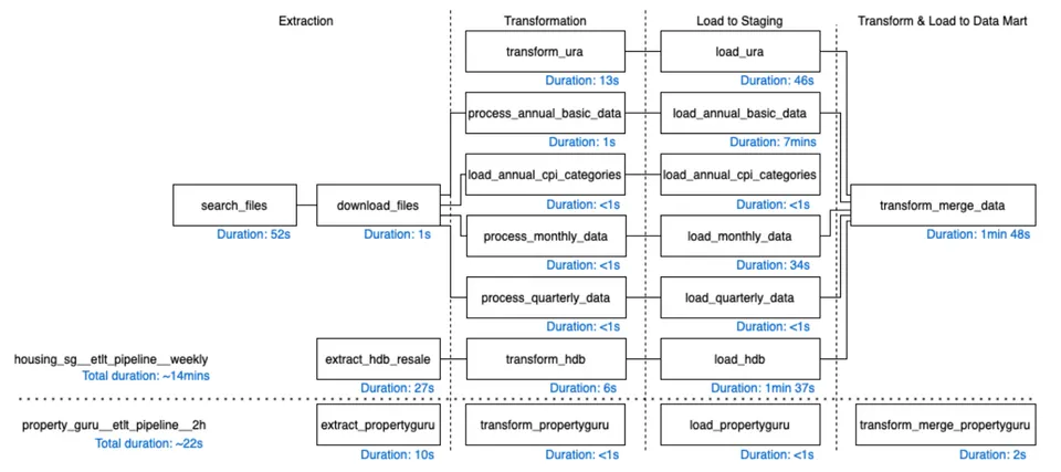
The workflow follows ETLT: Extract, Transform, Load, and Transform.

1. Extract: Retrieve HDB and SingStat data through APIs, read the compiled URA spreadsheets, and run the PropertyGuru browser scraper.
2. Initial transform: Clean column names, parse human-readable values, and standardise units and categories while preserving each dataset’s granularity.
3. Load: Load the cleaned sources into separate PostgreSQL staging tables.
4. Final transform: Merge and enrich compatible housing and economic records into a housing data mart, while keeping PropertyGuru listings in a separate data mart for model evaluation.

The housing data mart makes public and private transactions comparable through shared fields such as transaction date, district, property type, floor area, storey, remaining lease, price per square metre, and lagged economic indicators.

The two data marts support separate downstream workflows:

• Analysis and reporting: Use the housing data mart to generate price trends, correlation analysis, district comparisons, and breakdowns by lease, property type, and storey for the dashboard and PDF report.
• House-price prediction: Export the latest housing data each month, engineer features from floor area, storey, district, property age, remaining lease, income, interest rates, inflation, and other economic indicators, then compare linear, tree-based, ensemble, and time-series models. PropertyGuru asking prices from the separate data mart serve as a current-market evaluation set rather than training data.

The slower-moving transaction and economic datasets ran as weekly batches. PropertyGuru ran every two hours to collect a changing snapshot of asking prices, model training ran monthly, and reports could be generated from the latest stored data.

Transforming Inconsistent Sources

Each source needs its own staging path before the data can be merged.

For example, the HDB transformation turns values intended for human reading into model-ready features. Storey ranges become numerical midpoints, and remaining leases such as “52 years 3 months” become total months. Where the remaining lease is missing, it is derived from the transaction date, lease commencement date, and standard 99-year lease.

# "10 TO 12" -> 11.0
df["storey_range_continuous"] = df["storey_range"].apply(midpoint)

# "52 years 3 months" -> 627
df["remaining_lease_months"] = df["remaining_lease"].apply(to_months)

# null, transaction in 2020, lease starting in 1985 -> 768
df["remaining_lease_months"] = fill_missing(
    df["remaining_lease_months"],
    derive_remaining_lease(
        transaction_date=df["month"],
        lease_start=df["lease_commence_date"],
        original_lease_years=99,
    ),
)

# " MULTI-GENERATION " -> "multi generation"
df["flat_type"] = df["flat_type"].apply(normalise_category)

URA data arrives as manually compiled spreadsheets because the available interface does not support reliable bulk extraction. Tenure strings, floor ranges, property types, dates, and units are normalised before private transactions share a common schema with public housing data.

# "Transacted Price ($)" -> "transacted_price"
df = rename_to_common_schema(df)

# "Mar-25" -> 2025-03-01
df["sale_date"] = df["sale_date"].apply(parse_month_year)

# "06 to 10" -> 8.0
df["floor_level_continuous"] = df["floor_level"].apply(midpoint)

# "99 yrs lease from 2013", sold Mar 2025 -> 1,042
# "Freehold" -> 11,988, a consistent upper bound
df["remaining_lease_months"] = df.apply(parse_tenure, axis=1)

# 9 -> "D9", matching the other sources
df["postal_district"] = df["postal_district"].apply(prefix_district)

Staging the cleaned sources separately means more tables and tasks, but it preserves source-level granularity and makes a bad transformation easier to trace than it would be inside one large merge.

Scraping PropertyGuru

The scraper was the main technical challenge I owned.

I started with the requests library, which would have been the simplest and fastest way to approach the problem. PropertyGuru returned HTTP 403 responses to non-browser traffic, so that approach could not collect even the initial listings page.

I then moved to headless Selenium and ran Chrome inside the Airflow environment. This allowed the scraper to access the main property-for-sale page at https://www.propertyguru.com.sg/property-for-sale and extract listing IDs, titles, addresses, prices, agent descriptions, and the detail badges available on each card.

The browser solved access to the first page, but not the full collection problem. Opening individual listing pages (https://www.propertyguru.com.sg/listing/<listing_id>) or following pagination reliably triggered Cloudflare’s bot detection. Those routes offered a wider backlog and richer, more consistent property attributes, so losing them reduced both the number of observations and the depth of each record.

I experimented with undetected_chromedriver and Selenium stealth techniques, but neither made the deeper crawl dependable. Continuing to add evasion logic would have made the scraper more complex without giving the pipeline a stable data source.

After discussing the constraints with the team, we stopped trying to crawl the full site and chose a pragmatic middle ground: limiting the job to the first page gave us up to 20 of the newest listings every two hours.

This is a deliberate sampling strategy, not a complete PropertyGuru dataset. It makes the pipeline predictable enough to run for several days and supplies current asking prices for model evaluation without repeatedly failing on pagination.

The tradeoffs we had to accept were:

• Recency over representativeness: The first page captures what is new, not a balanced sample of property types, locations, or price bands.
• Reliability over feature depth: Listing cards expose enough fields for evaluation, but not everything available on a property’s detail page.
• Scheduled snapshots over complete history: Listings that appear and disappear between two-hour runs can be missed, while slower turnover can produce few new records.

Repeatedly scraping the first page also creates duplicates. We handled them by deduplicating on listing ID before loading the records into PostgreSQL.

The resulting PropertyGuru sample is therefore useful as a current-market check, but not as proof that the model generalises across the entire housing market.

Working with Delayed Economic Data

The newest property listings create another timing mismatch: several SingStat indicators only become available after the relevant calendar year, so a current listing cannot be paired with complete current-year economic data.

We considered training on same-year indicators and substituting older values only at prediction time. That would have given the model information during training that would not exist when making a real prediction.

Instead, we paired both training and evaluation records with one-year-lagged indicators. Experiments showed little performance difference from the unlagged version. The lag reduces apparent freshness, but it keeps training and inference consistent and prevents future information from leaking into the model.

One could argue that the relationship between economic indicators and housing prices is not instantaneous, so lagging the indicators may even be more realistic than using same-year values. However, the lag is a practical choice to avoid data leakage rather than a claim about market dynamics.

Analysis and Outputs

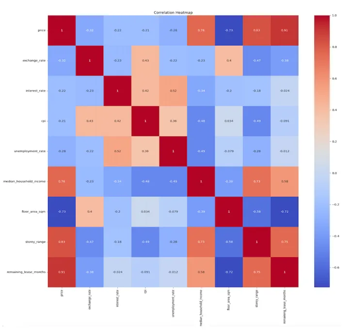
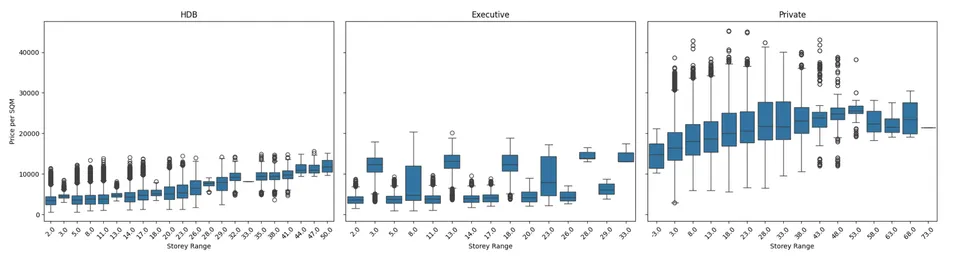
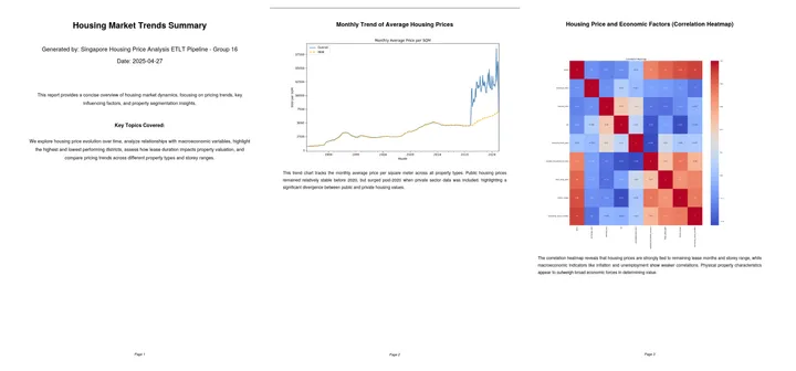
The clearest observed relationships are tied to the properties themselves. Longer remaining leases and higher storeys are associated with higher prices. Private properties occupy a higher and wider price range than HDB flats, while central districts have higher average prices than peripheral districts. Macroeconomic indicators such as inflation and unemployment show weaker correlations in this dataset.

House-Price Prediction Outputs

The final model blends XGBoost and LightGBM to predict a property’s price from its physical characteristics, location, and lagged economic context. Evaluation on the log-price scale produced an R² of 0.6324, while evaluation on the raw-price scale produced 0.0576. The results suggest that the model captures relative pricing patterns better than absolute errors across a market spanning ordinary HDB flats and high-value private properties.

These metrics also need to be read alongside the PropertyGuru sampling limitation. The scraped evaluation set is much smaller and less representative than the transaction data used for training, so it can reveal obvious model weaknesses but cannot establish robust performance across the full market.

The final outputs are:

• PostgreSQL data marts for housing analysis and PropertyGuru evaluation.
• A dashboard and generated PDF summarising housing trends and key relationships.
• Per-model PDF reports containing prediction plots and evaluation metrics.
• A FastAPI /predict endpoint exposing the serialised XGBoost-LightGBM pipeline.

Outcome

The final system connects API ingestion, spreadsheet processing, browser scraping, staged transformations, PostgreSQL storage, model training, and generated analysis in one scheduled Airflow environment.